Mass Definitions
hmf, as of v3.1, provides a simple way of converting between halo
mass definitions, which serves two basic purposes:
- the mass of a halo in one definition can be converted to its appropriate mass under another definition
- the halo mass function can be converted between mass definitions.
Introduction
By “mass definition” we mean the way the extent of a halo is defined. In
hmf, we support two main kinds of definition, which themselves can
contain different models. In brief, hmf supports Friends-of-Friends
(FoF) halos, which are defined via their linking length, \(b\), and
spherical-overdensity (SO) halos, which are defined by two criteria: an
overdensity \(\Delta_h\), and an indicator of what that overdensity
is with respect to (usually mean background density \(\rho_m\), or
critical density \(\rho_c\)). In addition to being able to provide a
precise overdensity for a SO halo, hmf provides a way to use the
so-called “virial” overdensity, as defined in Bryan and Norman (1998).
Converting between SO mass definitions is relatively simple: given a halo profile and concentration for the given halo mass, determine the concentration required to make that profile contain the desired density, and then compute the mass of the halo under such a concentration.
There is no clear way to perform such a conversion for FoF halos.
Nevertheless, if one assumes that all linked particles are the same
mass, and that halos are spherical and singular isothermal spheres (cf.
White (2001)), one can approximate an FoF halo by an SO halo of density
\(9 \rho_m /(2\pi b^3)\). hmf will make this approximation if a
conversion between mass definitions is desired.
Changing Mass Definitions
Most of the functionality concerning mass definitions is defined in the
hmf.halos.mass_definitions module:
In [1]:
import hmf
from hmf.halos import mass_definitions as md

print("Using hmf version v%s"%hmf.__version__)
Using hmf version v3.0.2
While we’re at it, import matplotlib and co:
In [2]:
import matplotlib.pyplot as plt
%matplotlib inline
import inspect
Different mass definitions exist inside the mass_definitions module
as Components. All definitions are subclassed from the abstract
MassDefinition class:
In [3]:
[x[1] for x in inspect.getmembers(md, inspect.isclass) if issubclass(x[1], md.MassDefinition)]
Out[3]:
[hmf.halos.mass_definitions.FOF,
 hmf.halos.mass_definitions.MassDefinition,
 hmf.halos.mass_definitions.SOCritical,
 hmf.halos.mass_definitions.SOMean,
 hmf.halos.mass_definitions.SOVirial,
 hmf.halos.mass_definitions.SphericalOverdensity]
The Mass Definition Component
To create an instance of any class, optional cosmo and z
arguments can be specified. By default, these are the Planck15
cosmology at redshift 0. We’ll leave them as default for this example.
Let’s define two mass definitions, both spherical-overdensity
definitions with respect to the mean background density:
In [4]:
mdef_1 = md.SOMean(overdensity=200)
mdef_2 = md.SOMean(overdensity=500)
Each mass definition has its own model_parameters, which define the
exact overdensity. For both the SOMean and SOCritical
definitions, the overdensity can be provided, as above (default is
200). This must be passed as a named argument. For the FOF
definition, the linking_length can be passed (default 0.2). For the
SOVirial, no parameters are available. Available parameters and
their defaults can be checked the same way as any Component within
hmf:
In [5]:
md.SOMean._defaults
Out[5]:
{'overdensity': 200}
The explicit halo density for a given mass definition can be accessed:
In [6]:
mdef_1.halo_density, mdef_1.halo_density/mdef_1.mean_density
Out[6]:
(17068502575484.857, 200.0)
Converting Masses
To convert a mass in one definition to a mass in another, use the following:
In [7]:
mnew, rnew, cnew = mdef_1.change_definition(m=1e12, mdef=mdef_2)
print("Mass in new definition is %.2f x 10^12 Msun / h"%(mnew/1e12))
print("Radius of halo in new definition is %.2f Mpc/h"%rnew)
print("Concentration of halo in new definition is %.2f"%cnew)
Mass in new definition is 0.76 x 10^12 Msun / h
Radius of halo in new definition is 0.16 Mpc/h
Concentration of halo in new definition is 4.81
The input mass argument can be a list or array of masses also. To convert between masses, the concentration of the input halos, and their density profile, must be known. By default, an NFW profile is assumed, with a concentration-mass relation from Duffy et al. (2008).
One can alternatively pass a concentration directly:
In [8]:
mnew, rnew, cnew = mdef_1.change_definition(m=1e12, mdef=mdef_2, c = 5.0)
print("Mass in new definition is %.2f x 10^12 Msun / h"%(mnew/1e12))
print("Radius of halo in new definition is %.2f Mpc/h"%rnew)
print("Concentration of halo in new definition is %.2f"%cnew)
Mass in new definition is 0.72 x 10^12 Msun / h
Radius of halo in new definition is 0.16 Mpc/h
Concentration of halo in new definition is 3.31
If you have halomod installed, you can also pass any
halomod.profiles.Profile instance (which itself includes a
concentration-mass relation) as the profile argument.
Converting Mass Functions
All halo mass function fits are measured using halos found using some
halo definition. While some fits explicitly include a parameterization
for the spherical overdensity of the halo (eg. Tinker08 and
Watson), others do not.
By passing a mass definition to the MassFunction constructor,
hmf will attempt to convert the mass function defined by the chosen
fitting function to the appropriate mass definition, by solving
for \(n'(m)\), resulting in
By default, the mass definition is None, which turns off all mass
conversion and uses whatever mass definition was employed by the chosen
fit. This keeps all existing code running as it was previously.
Nevertheless, care should be taken here: many of the different fits have
different mass definitions, and should not be compared without some form
of mass conversion. To see the mass definition intrinsic to the
measurement of each fit, use the following:
In [9]:
from hmf.mass_function.fitting_functions import SMT, Tinker08, Jenkins
In [10]:
print(SMT.sim_definition.halo_finder_type, SMT.sim_definition.halo_overdensity)
print(Tinker08.sim_definition.halo_finder_type, Tinker08.sim_definition.halo_overdensity)
print(Jenkins.sim_definition.halo_finder_type, Jenkins.sim_definition.halo_overdensity)
SO vir
SO *
FoF 0.2
Here “vir” corresponds to the virial definition of Bryan and Norman (1998), an asterisk indicates that the fit is itself parameterized for SO mass definitions, and 0.2 is the FoF linking length.
Let’s convert the mass definition of Tinker08, which has an
intrinsic parameterization:
In [21]:
# Default mass function object
mf = hmf.MassFunction()

dndm0 = mf.dndm

# Change the mass definition to 300rho_mean
mf.update(
    mdef_model  = "SOMean",
    mdef_params = {
        "overdensity": 300
    }
)

plt.plot(mf.m, mf.dndm/dndm0, label=r"300 $\rho_m$", lw=3)

# Change the mass definition to 500rho_crit
mf.update(
    mdef_model  = "SOCritical",
    mdef_params = {
        "overdensity": 500
    }
)

plt.plot(mf.m, mf.dndm/dndm0, label=r"500 $\rho_c$", lw=3)

plt.xscale('log')
plt.yscale('log')
plt.xlabel(r"Mass, $M_\odot/h$", fontsize=15)
plt.ylabel(r"Ratio of $dn/dm$ to $200 \rho_m$", fontsize=15)
plt.grid(True)
plt.legend();
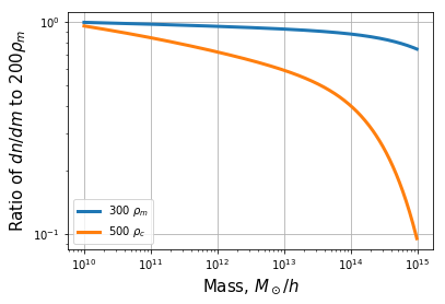
This did not require any internal conversion. Let’s try converting a fit that has no explicit parameterization for overdensity:
In [27]:
# Default mass function object.
mf = hmf.MassFunction(hmf_model = "SMT", Mmax=15)
dndm0 = mf.dndm

# Change the mass definition to 300rho_mean
mf.update(
    mdef_model  = "SOMean",
    mdef_params = {
        "overdensity": 300
    }
)
plt.plot(mf.m, mf.dndm/dndm0, label=r"300 $\rho_m$", lw=3)


# Change the mass definition to 500rho_crit
mf.update(
    mdef_model  = "SOCritical",
    mdef_params = {
        "overdensity": 500
    }
)
plt.plot(mf.m, mf.dndm/dndm0, label=r"500 $\rho_c$", lw=3)

plt.xscale('log')
plt.yscale('log')
plt.xlabel(r"Mass, $M_\odot/h$", fontsize=15)
plt.ylabel(r"Ratio of $dn/dm$ to virial", fontsize=15)
plt.grid(True)
plt.legend();
332.2445055922226 0.0
300
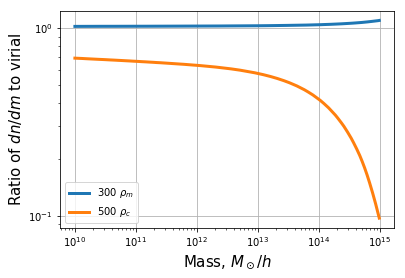
Here, the measured mass function uses “virial” halos, which have an overdensity of ~330\(\rho_m\), so that converting to 300\(\rho_m\) is a down-conversion of density. Finally, we convert a FoF mass function:
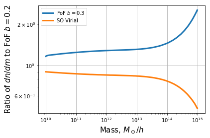
In [33]:
# Default mass function object.
mf = hmf.MassFunction(hmf_model = "Jenkins")
dndm0 = mf.dndm

# Change the mass definition to 300rho_mean
mf.update(
    mdef_model  = "FOF",
    mdef_params = {
        "linking_length": 0.3
    }
)
plt.plot(mf.m, mf.dndm/dndm0, label=r"FoF $b=0.3$", lw=3)


# Change the mass definition to 500rho_crit
mf.update(
    mdef_model  = "SOVirial",
    mdef_params = {}   # NOTE: we need to pass an empty dict here
                       # so that the "linking_length" argument is removed.
)
plt.plot(mf.m, mf.dndm/dndm0, label=r"SO Virial", lw=3)

plt.xscale('log')
plt.yscale('log')
plt.xlabel(r"Mass, $M_\odot/h$", fontsize=15)
plt.ylabel(r"Ratio of $dn/dm$ to FoF $b=0.2$", fontsize=15)
plt.grid(True)
plt.legend();